Section I:
Sampling Space and Manipulations
Now that we have a basic development environment set up, it would be prudent to review different methods for sampling and manipulating the coordinate system that dictates the output of our procedural processes. We will be basically reviewing built in functions to glsl that will help us in controlling our sampling space.
What is sampling space? You can think of it as the coordinate system/space that we will use as the value that we feed to our noise/procedural algorithms. This can be anything that effectively want from a singular value to a n-dimensional location…. In most of our cases we will be using the vPosition or the vUV as our coordinate space, even though there are other special situations that may dictate you use a difference system. You can review this concept starting on page 24 of [1] where they explain coordinate space with these points:
• The current space is the one in which shading calculations are normally done.
In most renderers, current space will turn out to be either camera space or
world space, but you shouldn’t depend on this.

• The world space is the coordinate system in which the overall layout of your
scene is defined. It is the starting point for all other spaces.

• The object space is the one in which the surface being shaded was defined. For
instance, if the shader is shading a sphere, the object space of the sphere is the
coordinate system that was in effect when the RiSphere call was made to create
the sphere. Note that an object made up of several surfaces all using the same
shader might have different object spaces for each of the surfaces if there are
geometric transformations between the surfaces.

• The shader space is the coordinate system that existed when the shader was in-
voked (e.g., by an RiSurface call). This is a very useful space because it can be
attached to a user-defined collection of surfaces at an appropriate point in the
hierarchy of the geometric model so that all of the related surfaces share the
same shader space.
Which if you ask me is overkill on the explanation. It all boils down to what values you choose to reference when feeding out procedural algorithms. If we have a 3d noise for example we would most likely use the vPosition which is an xyz value for that pixels location in the 3d scene locally, if you used gl_FragCoord, I believe that would be global (do not quote me on this). By making some quick changes to our page and changing the argument that we initialize the objects fragment shader to something like this:
precision highp float;
//Varyings
varying vec2 vUV;

void main(void) {
    vec3 color = vec3(vUV.x, vUV.y, vUV.y);
    gl_FragColor = vec4(color, 1.0);
}
With everything in its place we can see now when we refresh the page, a gradient that should look like this:
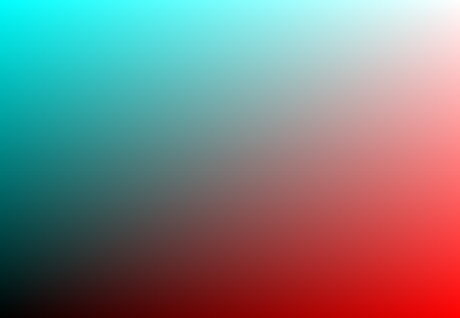
What this is showing us is that our UV is set up correctly, as the lower left corner is black where vUV.x & vUV.y == 0; white where they are 1; Red where x is 1 & y is 0; and finally Cyan where y is 1 and x is 0. We are directly effecting the color by the uv values our very first procedural (explicit) texture!
Modulate
Now that we can have established our coordinate space, how can me manipulate it do to our biding.
There is a collection of methods available to us in glsl, but lets take a look at which ones [1] mentions starting on page 27.
step
Description:
step generates a step function by comparing x to edge.
For element i of the return value, 0.0 is returned if x[i] < edge[i], and 1.0 is returned otherwise.
We can also define a method that uses the step function to generate what is known as a pulse by doing the following:
float pulse(float a, float b, float v){
return step(a,v) – step(b,v);
}
Which makes everything outside of the range between a-b come up as 1 and anything outside as 0. This gives us the ability to effectively create a rectangle in what ever range we decide.
clamp
Description:
clamp returns the value of x constrained to the range minVal to maxVal. The returned value is computed as min(max(x, minVal), maxVal).
The next method does not have much use unless you are using a coordinate system that has negative values. Normally for sampling coordinates you will want to work in a -1 to 1 range and not a 0 to 1 range, so lets adjust the default vertex shader to have a new varying variable that has the uv transposed to this range.
...
vx:
`precision highp float;
//Attributes
attribute vec3 position;
attribute vec2 uv;
// Uniforms
uniform mat4 worldViewProjection;
//Varyings
varying vec2 vUV;
varying vec2 tUV;

void main(void) {
    vec4 p = vec4( position, 1. );
    gl_Position = worldViewProjection * p;
    vUV = uv;
    tUV = uv*2.0-1.0;
}`,
...
abs
Description:
abs returns the absolute value of x.
smoothstep
Description:
smoothstep performs smooth Hermite interpolation between 0 and 1 when edge0 < x < edge1. This is useful in cases where a threshold function with a smooth transition is desired. smoothstep is equivalent to:
genType t; /* Or genDType t; */
t = clamp((x - edge0) / (edge1 - edge0), 0.0, 1.0);
return t * t * (3.0 - 2.0 * t);
Results are undefined if edge0 ≥ edge1.
mod
Description:
mod returns the value of x modulo y. This is computed as x – y * floor(x/y).
With the mod method and the pulse function that we created, we can now create another function to create a “pulsate” function
References
1. TEXTURING & MODELING – A Procedural Approach (third edition)
gamma
Description:
The zero and one end points of the interval are mapped to themselves. Other values are shifted upward toward one if gamma is greater than one, and shifted downward toward zero if gamma is between zero and one.[1]
bias
Description:
Perlin and Hoffert (1989) use a version of the gamma correction function that they call the bias function.[1]
gain
Description:
Regardless of the value of g, all gain functions return 0.5 when x is 0.5. Above and below 0.5, the gain function consists of two scaled-down bias curves forming an S-shaped curve. Figure 2.20 shows the shape of the gain function for different choices of g.[1]
There are quite a few more (sin, cos, tan, etc) but we will cover those more later, if you want to go over more now check out: http://www.shaderific.com/glsl-functions/. These that I have presented here though should be enough to start making some more dynamic of sampling spaces. With all this at our disposal what is something that we could make of use? A pretty standard texture in the procedural world would be a brick or checkerboard pattern, so lets start there.
Oh Bricks
Shamelessly this is a reproduction of the bricks presented in [1] (page 39) with a few changes made. Before creating anything lets take a look at what identifiable elements that we are trying to produce. A brick of course and its size in relation to the whole element, the mortar or padding around it and then its offset in relation to the other rows. To get started lets define a few variables (on the fx fragment we are passing to the SM object) to define the number of bricks we wish to see. This is different then our reference script but I feel is easier to understand and we can derive all our other size numbers from them. Plus there is the added advantage doing it this way, we can make sure the texture is repeatable on all sides.
...
#define XBRICKS 2.
#define YBRICKS 4.
#define MWIDTH 0.1

void main(void) {
...
Super simple right? We define the counts as floats for simplicity cause who likes working with integers and having to convert them every time you want to do quick maths, heh…. Now that we have the basic numbers to base everything off of lets set up some colors and then get our sampling space into scope.
...
void main(void) {
    vec3 brickColor = vec3(1.,0.,0.);
    vec3 mortColor = vec3(0.55);

    vec2 brickSize = vec2(
    	1.0/XBRICKS,
    	1.0/YBRICKS
    );

    vec2 pos = vUV/brickSize;

    if(fract(pos.y * 0.5) > 0.5){
     	pos.x += 0.5;
    }

    pos = fract(pos);

    float x = pos.x;
    float y = pos.y;
    vec3 color = vec3(x, y, y);
    gl_FragColor = vec4(color, 1.0);
}
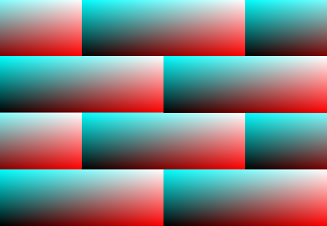
Now we have set up our sampling space by first dividing our max coordinate unit by the brick count. Then we divide the coordinate space we are using by the brick size. This would give us coordinate space that now has values ranging from 0 to the number of bricks we accounted for. After checking the vertical positions fractional half value and seeing if it is over 0.5 we are able to identify the alternating rows, which we then offset the x position by half of the coordinate space. Then we transpose the position range because the only thing we are worried about in this range is the fractional sections of the values not the whole number. The mortar size we will take into account after the bricks are in place so that way we can keep the padding around the bricks constant by using some ratio calculations.
If you are following along and refresh your page now you should see an image similar to:
Now with this basic grid set up, we can take into consideration the position of our mortar around the bricks and start the process of coloring everything. A quick way to figure this out will be to just define a vec2 with our mortar size, then do a quick step calculation on our set up coordinate space to see if its brick or not. We then mix the brick and mortar colors together with the mix value being set as the result of multiplying the step calculation we just made. The cool thing about the step multiplication is it will turn the mix value to 0 anytime the step calculation are outside of the brick area.
...
void main(void) {
    vec3 brickColor = vec3(1.,0.,0.);
    vec3 mortColor = vec3(0.55);

    vec2 brickSize = vec2(
    	1.0/XBRICKS,
    	1.0/YBRICKS
    );

    vec2 pos = vUV/brickSize;
    vec2 mortSize = vec2(MWIDTH);

    if(fract(pos.y * 0.5) > 0.5){
     	pos.x += 0.5;
    }

    pos = fract(pos);

    vec2 brickOrMort = step(pos, mortSize);

    vec3 color =  mix(mortColor, brickColor, brickOrMort.x * brickOrMort.y);

    gl_FragColor = vec4(color, 1.0);
}
If we refresh now, we will see it is close but no cigar… why is this? I quick hint would be that it seems the mortar value must be off, and I know this is a crap explanation but just by looking at it I knew the solution was to inverse value so our mortSize line becomes:
...
    vec2 mortSize = 1.0-vec2(MWIDTH);
...
With a page reload we now see something like this:
Getting closer! The first thing that we notice is the mortar is thicker on it height vs width ratio. This is super easy to fix by manipulating our mortSize to reflect the same ratio of bricks x:y.
Making our variable become:
...
    vec2 mortSize = 1.0-vec2(MWIDTH*(XBRICKS/YBRICKS), MWIDTH);
...
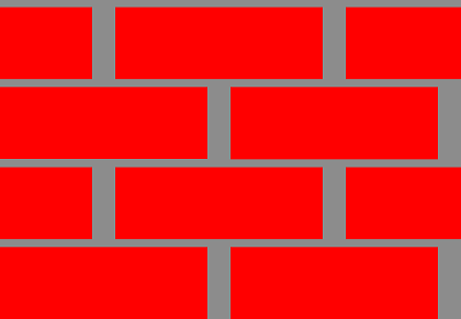
This will make our mortar lines keep the same padding around the bricks and makes our procedural texture almost complete! The one last thing I would like to add would be an offset of the entire coordinate space to shift both the rows and columns by half of the mortar size in order to “center” the repetition properties of this texture. It is a optional line and is up to the developer to decide if they want to use it or not!
...
    vec2 mortSize = 1.0-vec2(MWIDTH*(XBRICKS/YBRICKS), MWIDTH);
    pos += mortSize*0.5;
...
Thats it for now! You have officially created your first real procedural texture, not just a gradient or a solid color. This shader can now be extended upon and made way more dynamic. If you are having trouble getting good results please reference or download the Example
This concludes this section, in the next one we will discuss setting up controls and parameters for real time manipulation of the texture to debug/test different values.
Continue to Section II
References
1. TEXTURING & MODELING – A Procedural Approach (third edition)
