Section IV
Getting Noisy in Here
Finally the part I have been wanting to get to! One of the power players in the procedural world are methods called noise. Noise is a random (in our case pseudorandom) distribution of values over a range. Normally these values range from -1 to 1, but can have other values. We use these predictably random functions to control our methods. The simplest, yet least useful to use will be a white noise function, which some of you should be familiar with. Picture your old analog TV set to a blank channel or the scene from the movie Poltergeist.
Example
There has been quite a bit of advancement in the generation of random values, with the works of Steven Worley and Ken Perlin. We can use a combination of their methods, to achieve some really interesting results. The are two main types of noise that we will be covering are lattice and gradient based noise methods.
Lattice Noise/Value Noise
There is a little bit of confusion in the procedural world with what is a value based noise and what is gradient. This is demonstrated by the article we will be referencing calls the process we will be reviewing [1] Perlin when it is actually Value Noise.
Value Noise is a series of nDimensional points at a set frequency that have a value, we then interpolate between the points which then gives us our values. There are multiple ways to interpolate the values and most do it smoothly but to help you understand the concept lets temporarily do a linear interpolation.
Take for example if we had a 1D noise with our lattice set at every integer value and a linear interpolation we get a graph similar to this:
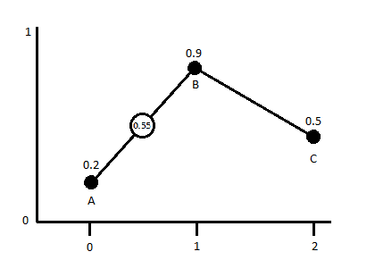
If we were to sample any point now between any of the lattice points we would get a value between the values of the closets points. In this 1d grid it would be the two closest points, in a 2d grid it would be 4 and in a 3d grid it would be 6 (for 2d/3d you can sample more but these are the minimum neighborhoods). So if we were to sample from this 1d Noise at the coordinate x=1.5 we would end up with a value of 0.55 (unless my math sucks).
If we use this process and mix together value noises of increasing frequency and decreasing amplitude we can make some interesting results. Another parameter we can introduce for control is persistence, which has some confusion as well as to its “official” definition. The term was first used by Mandelbrot while developing fractal systems. The simplest way to describe it would be the weighted effect of the values on the sum of the noise functions.
Random Function
In order to get our noise functions rolling we first need to create a random number generation method. Here is a section of pseudo-code presented in [1]:
function IntNoise(32-bit integer: x) x = (x<<13) ^ x; return ( 1.0 - ( (x * (x * x * 15731 + 789221) + 1376312589) & 7fffffff) / 1073741824.0); end IntNoise function
Right away one should notice that this is very close to the code that we used for the white noise generator above. There are many ways to generate a random number but we will convert this one initially and then test other methods to see which are more effective.
The GLSL version of this code would be:
float rValueInt(int x){
    x = (x >> 13) ^ x;
    int xx = (x * (x * x * 60493 + 19990303) + 1376312589) & 0x7fffffff;
    return 1.0 - (float(xx) / 1073741824.0);
}
This function requires our input value to be an integer (hence making it a lattice), we then use bit-wise operators as explained in GLSL specs[2]. I have no clue what is really happening with the bit-wise stuff other then we are shifting the number around… sorry I dont know more. The numbers that we used are right from Hugos example [1] and are prime numbers. You can change these numbers all you want, just make sure you keep them as prime in order to prevent as noticeable of graphic artifacts. From here we just need to decide how we want to interpolate the values between points.
Its all up to Interpolation…
The simplest way to interpolate is linearly like what we used above is represented by this equation:
Mock CodeGLSL Code
function Linear_Interpolate(a, b, x)
	return  a*(1-x) + b*x
  end of function
float linearInterp(float a, float b, float x){
	return a*(1.-x) + b*x;
}
This is ok if we want sharp elements, but if we want smoother transitions we can use a cosine interpolation.
function Cosine_Interpolate(a, b, x)
    ft = x * 3.1415927
    f = (1 - cos(ft)) * .5
    return  a*(1-f) + b*f
end of function
float cosInterp(float a, float b, float x){
	float ft = x*3.12159276;
	float f = (1.0 - cos(ft)) * .5;
	return a*(1.-f) + b*f;
}
There is also cubic iterp, but we will skip that for now and focus on linear and cosine. The last thing we will want to do, in order to make our noises smoother on their transitions is introduce a you guessed it smoothing function. This function can optionally be used and can be expanded to how ever many dimensions you would need. The smoothing helps reduce the appearance of block artifacts when rendering out to 2+ dimensions. Here is a snip-it of pseudo-code from [1].
//1-dimensional Smooth Noise
  function Noise(x)
    ...    .
  end function

  function SmoothNoise_1D(x)
    return Noise(x)/2  +  Noise(x-1)/4  +  Noise(x+1)/4
  end function
//2-dimensional Smooth Noise
function Noise(x, y)
...
end function

function SmoothNoise_2D(x>, y)

    corners = ( Noise(x-1, y-1)+Noise(x+1, y-1)+Noise(x-1, y+1)+Noise(x+1, y+1) ) / 16
    sides   = ( Noise(x-1, y)  +Noise(x+1, y)  +Noise(x, y-1)  +Noise(x, y+1) ) /  8
    center  =  Noise(x, y) / 4

    return corners + sides + center

end function
Later in this section we will look at the differences between smoothed and non-smoothed noise. Now we need to start taking all these elements and put them together. Here is the pseudo code as exampled by [1]
function Noise1(integer x) x = (x<<13) ^ x; return ( 1.0 - ( (x * (x * x * 15731 + 789221) + 1376312589) & 7fffffff) / 1073741824.0); end function function SmoothedNoise_1(float x) return Noise(x)/2 + Noise(x-1)/4 + Noise(x+1)/4 end function function InterpolatedNoise_1(float x) integer_X = int(x) fractional_X = x - integer_X v1 = SmoothedNoise1(integer_X) v2 = SmoothedNoise1(integer_X + 1) return Interpolate(v1 , v2 , fractional_X) end function function PerlinNoise_1D(float x) total = 0 p = persistence n = Number_Of_Octaves - 1 loop i from 0 to n frequency = 2i amplitude = pi total = total + InterpolatedNoisei(x * frequency) * amplitude end of i loop return total end function
I decided to make a few structural changes to this for the GLSL conversion. In the above example they use four functions to make it happen, we are going to do it with three. I think it will also be relevant to add uniforms (or defines depends on your preference) to control things like octaves, persistence and a smoothness toggle. I will also be using strictly the cos interpolation, this is by personal choice any method can be used though. So following the structure of our SM object, we set up the shader argument as follows:
sm = new SM(
{
size : new BABYLON.Vector2(512, 512),
hasTime : false,
//timeFactor : 0.1,
uniforms:{
	octaves:{
		type : 'float',
		value : 4,
		min : 0,
		max : 124,
		step: 1,
		hasControl : true
	},
	persistence:{
		type : 'float',
		value : 0.5,
		min : 0.001,
		max : 1.0,
		step: 0.001,
		hasControl : true
	},
	smoothed:{
		type : 'float',
		value : 1.0,
		min : 0,
		max : 1.0,
		step: 1,
		hasControl : true
	},
	zoom:{
		type : 'float',
		value : 1,
		min : 0.001,
		step: 0.1,
		hasControl : true
	},
	offset:{
		type : 'vec2',
		value : new BABYLON.Vector2(0, 0),
		step: new BABYLON.Vector2(1, 1),
		hasControl : true
	},
},
fx :
`precision highp float;
//Varyings
varying vec2 vUV;
varying vec2 tUV;
/*----- UNIFORMS ------*/
uniform float time;
uniform vec2 tSize;
uniform float octaves;
uniform float persistence;
uniform float smoothed;
uniform float zoom;
uniform vec2 offset;
This will set up all of our uniforms and the defaults for them. You can do these as defines, but if having the ability to manipulate it on the fly they should be uniforms. I also added a uniform that we will not be manipulating directly ever but letting the size of the canvas/texture set this value when the shader is compiled. With this we need to make some changes to our SM object to accommodate this new uniform.
SM = function(args, scene){
	...
	this.buildGUI();

	this.setSize(args.size);

	return this;
}

SM.prototype = {
...
setSize : function(size){
	var canvas = this.scene._engine._gl.canvas;
	size = size || new BABYLON.Vector2(canvas.width, canvas.height);
	this._size = size;
	var pNode = canvas.parentNode;
	pNode.style.width = size.x+'px';
	pNode.style.height = size.y+'px';
	this.scene._engine.resize();
	this.buildOutput();
	this.buildShader();
}
...
Now the shader will always know what the size of the texture is, because we have made this a inherent feature of the SM object we need to add the uniform for tSize to the default fragment that the shader has built in. This is in the situation that the default shader get bound that it will validate and compile. From here we need to include our random number function, our interpolation function and the noise function itself. I am going to include a lerp function as well in case you want to use this and the interpolation vs cos.
//Methods
//1D Random Value from INT;
float rValueInt(int x){
	x = (x >> 13) ^ x;
	int xx = (x * (x * x * 60493 + 19990303) + 1376312589) & 0x7fffffff;
	return 1. - (float(xx) / 1073741824.0);
}
//float Lerp
float linearInterp(float a, float b, float x){
	return a*(1.-x) + b*x;
}
//float Cosine_Interp
float cosInterp(float a, float b, float x){
	float ft = x*3.12159276;
	float f = (1.0 - cos(ft)) * .5;
	return a*(1.-f) + b*f;
}
//1d Lattice Noise
float valueNoise1D(float x, float persistence, float octaves, float smoothed){
float t = 0.0;
float p = persistence;
float frequency, amplitude, tt, v1, v2, fx;
int ix;
for(float i=1.0; i<=octaves; i++){
	frequency = i*2.0;
	amplitude = p*i;

	ix = int(x*frequency);
	fx = fract(x*frequency);

	if(smoothed > 0.0){
		v1 = rValueInt(ix)/2.0 + rValueInt(ix-1)/4.0 + rValueInt(ix+1)/4.0;
		v2 = rValueInt(ix+1)/2.0 + rValueInt(ix)/4.0 + rValueInt(ix+2)/4.0;
		tt = cosInterp(v1, v2, fx);
	}else{
		tt = cosInterp(rValueInt(ix), rValueInt(ix+1), fx);
	}

	t+= tt*amplitude;
}
t/=octaves;
return t;
}
So now we have a GLSL function to generate some 1D noise! It has four arguments, the last one of smoothed can be omitted if you please but I like having it so…. It a fairly simple function and most of our noise functions will have a similar structure. We could also put a #define in that would control the interpolation, but for simplicity I am just using the cosine method. From here it is as simple as setting up the main function of our shader program to use this noise. To do this we decide our sampling space and pass that to the x value of the noise function along with our other uniforms that we have already set up.
void main(void) {
	vec2 tPos = ((vUV*tSize)+offset)/zoom;
	float v = valueNoise1D(tPos.x, persistence, octaves, smoothed)+1.0/2.0;
	vec3 color = vec3(mix(vec3(0.0), vec3(1.0), v));
    gl_FragColor = vec4(color, 1.0);
}
Super easy right!? Our sampling space that we use is the 0-1 uv multiplied by the size of the texture, which effectively shifts us to texel space. The choice to use to vUV instead of the tUV was because for some reason the negative value was creating an artifact as seen here: 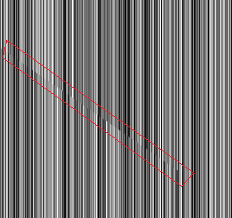
I could try to trouble shoot that, but instead its just easier to use the 0-1 uv range and move on.
Next add an offset which is also in texel space, you could do it as a percentage of the texture’s size but that is user preference. We then divide the whole thing by a zoom value. That gives us a nice sampling space, which we then pass to our noise function with our other arguments. Because the noise function returns a number between negative 1 and positive 1, we shift it to a 0-1 range by simply adding one then dividing the sum by two.
A New Dimension
One dimensional noise is cool and has its uses, but we need more room for activities. Before we develop more noises and look at different methods for generation having an understanding of how to extend the noise to n-dimensions is pretty important. For all general purposes all calculations stay the same, you just have to make a couple more of them. It would probably be smart to add a support function for smoothing the values of the interpolation now that we are working with larger dimensions. The main modifications to the function will be changing some of the variables from floats and integers to vectors of the same type. The last function to add is a random number generator that takes into consideration the 2 dimensions.
//2D Random Value from INT vec2;
float rValueInt(ivec2 p){
	int x = p.x, y=p.y;
	int n = x+y*57;
	n = (n >> 13) ^ n;
	int nn = (n * (n * n * 60493 + 19990303) + 1376312589) & 0x7fffffff;
	return 1. - (float(nn) / 1073741824.0);
}

float smoothed2dVN(ivec2 pos){
return (( rValueInt(pos+ivec2(-1))+ rValueInt(pos+ivec2(1, -1))+rValueInt(pos+ivec2(-1, 1))+rValueInt(pos+ivec2(1, 1)) ) / 16.) + //corners
	   (( rValueInt(pos+ivec2(-1, 0)) + rValueInt(pos+ivec2(1, 0)) + rValueInt(pos+ivec2(0, -1)) + rValueInt(pos+ivec2(0,1)) ) / 8.) + //sides
	   (rValueInt(pos) / 4.);
}

//2d Lattice Noise
float valueNoise(vec2 pos, float persistence, float octaves, float smoothed){
float t = 0.0;
float p = persistence;
float frequency, amplitude, tt, v1, v2, v3, v4;
vec2 fpos;
ivec2 ipos;
for(float i=1.0; i<=octaves; i++){
	frequency = i*2.0;
	amplitude = p*i;

	ipos = ivec2(int(pos.x*frequency), int(pos.y*frequency));
	fpos =  vec2(fract(pos.x*frequency), fract(pos.y*frequency));

	if(smoothed > 0.0){
		ivec2 oPos = ipos;
		v1 = smoothed2dVN(oPos);
		oPos = ipos+ivec2(1, 0);
		v2 = smoothed2dVN(oPos);
		oPos = ipos+ivec2(0, 1);
		v3 = smoothed2dVN(oPos);
		oPos = ipos+ivec2(1, 1);
		v4 = smoothed2dVN(oPos);

		float i1 = cosInterp(v1, v2, fpos.x);
		float i2 = cosInterp(v3, v4, fpos.x);
		tt = cosInterp(i1, i2, fpos.y);

	}else{
		float i1 = cosInterp(rValueInt(ipos), rValueInt(ipos+ivec2(1,0)), fpos.x);
		float i2 = cosInterp(rValueInt(ipos+ivec2(0,1)), rValueInt(ipos+ivec2(1,1)), fpos.x);

		tt = cosInterp(i1, i2, fpos.y);
	}

	t+= tt*amplitude;
}
t/=octaves;
return t;
}
There we have it, there are definitely some problems with this method that if we took some time and refined this could be fixed. These problems are things like artifacts as the noise transfers from a positive to a negative coordinate range which is apparent the more you zoom in and noticeable circular patterns the closer to 0,0 we get. In order to fix this quickly and essentially ‘ignore’ that problem we just add a large offset to the noise initially and screw our coordinates to be far away from the artifacts.
As a challenge see if you can change the interpolation function to be cubic. Read the section on it here [3].
You can also see a live example of the 2d Lattice Noise here.
Better Noise from Gradients
References
1. Hugo Elia’s “Perlin noise” implementation. Value Noise, mislabeled as Perlin noise.
2. https://www.khronos.org/registry/OpenGL/specs/gl/GLSLangSpec.1.20.pdf
3. C# Noise
